| sepal_length | sepal_width | petal_length | petal_width | species | |
|---|---|---|---|---|---|
| 0 | 5.1 | 3.5 | 1.4 | 0.2 | Iris-setosa |
| 1 | 4.9 | 3.0 | 1.4 | 0.2 | Iris-setosa |
| 2 | 4.7 | 3.2 | 1.3 | 0.2 | Iris-setosa |
| 3 | 4.6 | 3.1 | 1.5 | 0.2 | Iris-setosa |
| 4 | 5.0 | 3.6 | 1.4 | 0.2 | Iris-setosa |
Data Analysis of Iris Dataset
About
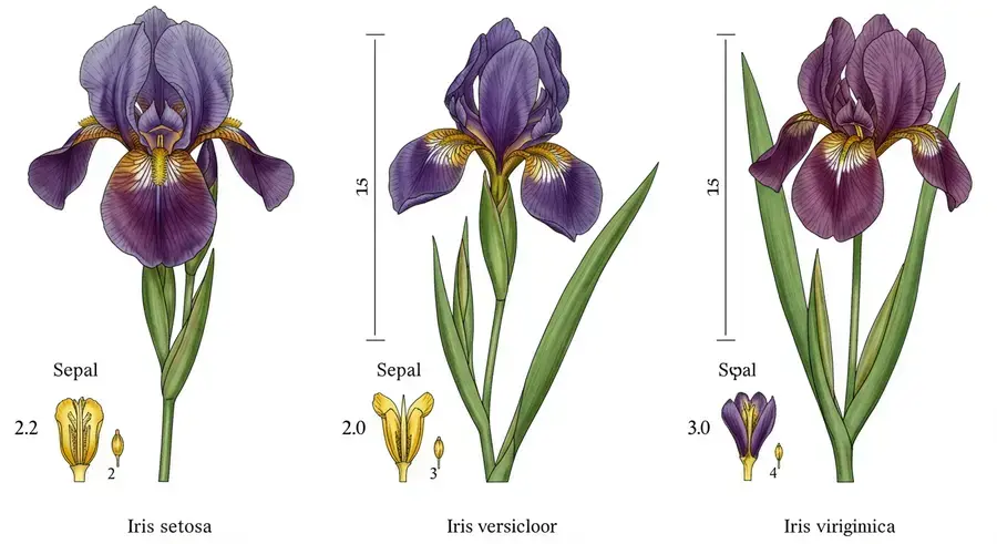
The Iris dataset is a small but famous dataset used since 1936 to demonstrate classification techniques. It contains 150 samples of three Iris species, each with 50 observations:
- Iris setosa
- Iris versicolor
- Iris virginica
For each flower, four morphological features were measured:
- Sepal length (cm)
- Sepal width (cm)
- Petal length (cm)
- Petal width (cm)
You can downloaded dataset here
Loading Data
Description of Dataset
<class 'pandas.core.frame.DataFrame'>
RangeIndex: 150 entries, 0 to 149
Data columns (total 5 columns):
 #   Column        Non-Null Count  Dtype
---  ------        --------------  -----
 0   sepal_length  150 non-null    float64
 1   sepal_width   150 non-null    float64
 2   petal_length  150 non-null    float64
 3   petal_width   150 non-null    float64
 4   species       150 non-null    object
dtypes: float64(4), object(1)
memory usage: 6.0+ KBNone| count | mean | std | min | 25% | 50% | 75% | max | |
|---|---|---|---|---|---|---|---|---|
| sepal_length | 150.0 | 5.843333 | 0.828066 | 4.3 | 5.1 | 5.80 | 6.4 | 7.9 |
| sepal_width | 150.0 | 3.054000 | 0.433594 | 2.0 | 2.8 | 3.00 | 3.3 | 4.4 |
| petal_length | 150.0 | 3.758667 | 1.764420 | 1.0 | 1.6 | 4.35 | 5.1 | 6.9 |
| petal_width | 150.0 | 1.198667 | 0.763161 | 0.1 | 0.3 | 1.30 | 1.8 | 2.5 |
Checking Data Quality
Missing values per column:
 sepal_length    0
sepal_width     0
petal_length    0
petal_width     0
species         0
dtype: int64
Duplicate rows: 3
I have not found any missing values. Duplicates reflect real repeated values in the source.
Summaries
Summaries for features:
count    150.000000
mean       5.843333
std        0.828066
min        4.300000
25%        5.100000
50%        5.800000
75%        6.400000
max        7.900000
Name: sepal_length, dtype: float64
count 150.000000
mean 3.054000
std 0.433594
min 2.000000
25% 2.800000
50% 3.000000
75% 3.300000
max 4.400000
Name: sepal_width, dtype: float64count 150.000000
mean 3.758667
std 1.764420
min 1.000000
25% 1.600000
50% 4.350000
75% 5.100000
max 6.900000
Name: petal_length, dtype: float64count 150.000000
mean 1.198667
std 0.763161
min 0.100000
25% 0.300000
50% 1.300000
75% 1.800000
max 2.500000
Name: petal_width, dtype: float64Summaries for species:
Summary for species: Iris-setosa
| count | mean | std | min | 25% | 50% | 75% | max | |
|---|---|---|---|---|---|---|---|---|
| sepal_length | 50.0 | 5.006 | 0.352490 | 4.3 | 4.800 | 5.0 | 5.200 | 5.8 |
| sepal_width | 50.0 | 3.418 | 0.381024 | 2.3 | 3.125 | 3.4 | 3.675 | 4.4 |
| petal_length | 50.0 | 1.464 | 0.173511 | 1.0 | 1.400 | 1.5 | 1.575 | 1.9 |
| petal_width | 50.0 | 0.244 | 0.107210 | 0.1 | 0.200 | 0.2 | 0.300 | 0.6 |
Summary for species: Iris-versicolor
| count | mean | std | min | 25% | 50% | 75% | max | |
|---|---|---|---|---|---|---|---|---|
| sepal_length | 50.0 | 5.936 | 0.516171 | 4.9 | 5.600 | 5.90 | 6.3 | 7.0 |
| sepal_width | 50.0 | 2.770 | 0.313798 | 2.0 | 2.525 | 2.80 | 3.0 | 3.4 |
| petal_length | 50.0 | 4.260 | 0.469911 | 3.0 | 4.000 | 4.35 | 4.6 | 5.1 |
| petal_width | 50.0 | 1.326 | 0.197753 | 1.0 | 1.200 | 1.30 | 1.5 | 1.8 |
Summary for species: Iris-virginica
| count | mean | std | min | 25% | 50% | 75% | max | |
|---|---|---|---|---|---|---|---|---|
| sepal_length | 50.0 | 6.588 | 0.635880 | 4.9 | 6.225 | 6.50 | 6.900 | 7.9 |
| sepal_width | 50.0 | 2.974 | 0.322497 | 2.2 | 2.800 | 3.00 | 3.175 | 3.8 |
| petal_length | 50.0 | 5.552 | 0.551895 | 4.5 | 5.100 | 5.55 | 5.875 | 6.9 |
| petal_width | 50.0 | 2.026 | 0.274650 | 1.4 | 1.800 | 2.00 | 2.300 | 2.5 |
Exploratory Data Analysis
Histograms of Morphological Values
Histogram is the plot that shows distribution of values. I decided to add lines of kernel density estimation that smooths data distribution for each species of Iris for better data representation.
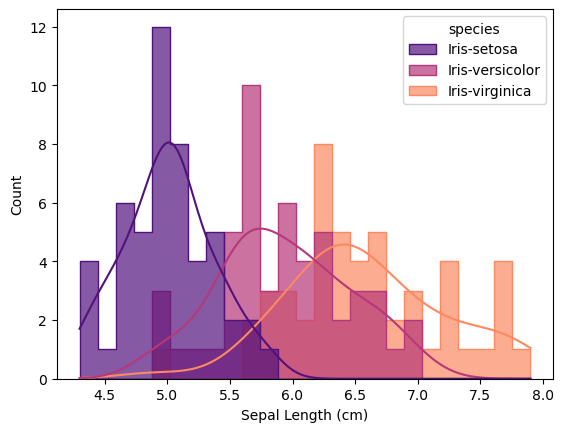
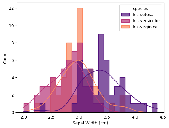
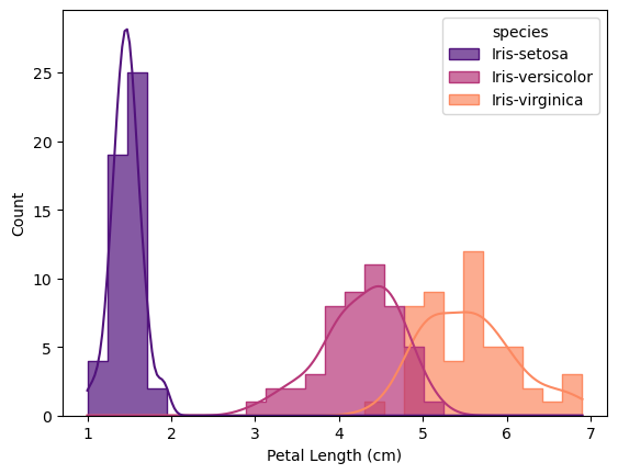
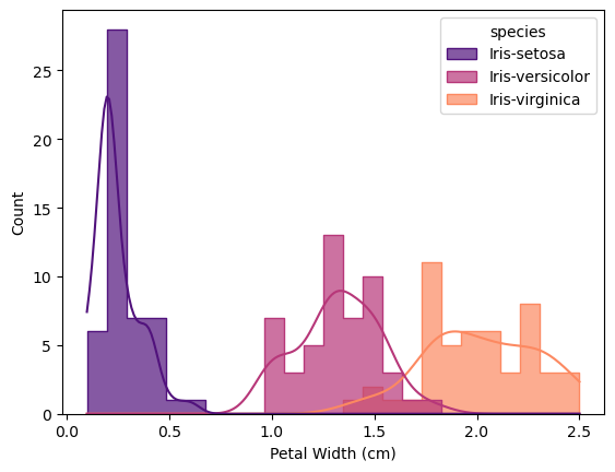
According to histograms, flowers of Iris Virginica and Iris Versicolor share similar values, with mean value for Iris Virginica’s flowers higher in any category than for flowers of Iris Versicolor. Flowers of Iris Setosa differ from these species with lower values for petal length, petal width, sepal length, but higher values for sepal width than for Iris Virginica and Iris Versicolor. All histograms are saved in the folder histograms.
Violin Plots
The violin plot combines the information of the boxplot and the density plot. The “violins” show the full distribution of a features for each Iris species, while also marking the medians and quartiles.
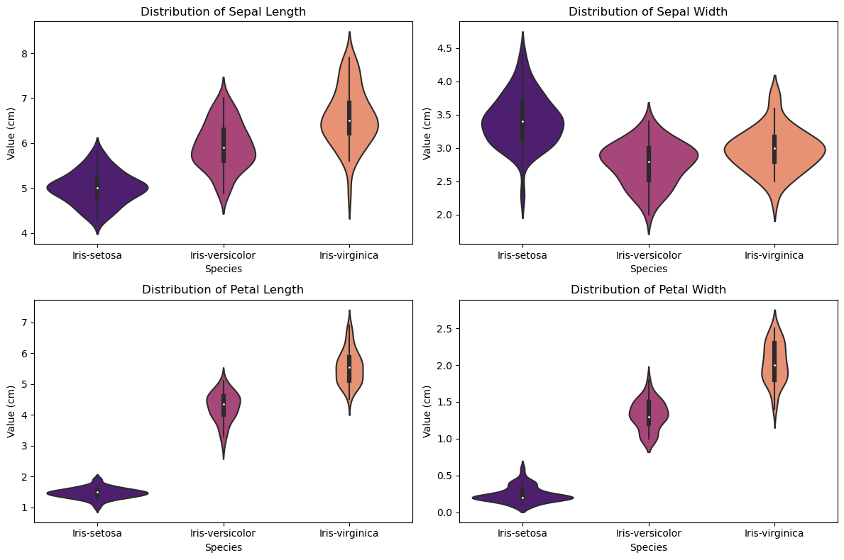
For petal length and width, Setosa is completely separated from the other two species, which is consistent with histograms.
Versicolor and Virginica overlap, though Virginica generally has larger values.
For sepal length and width, all three species overlap more, showing these features are less useful for classification.
Overall, violin plots confirm that petal features carry the strongest discriminatory power.
Correlation Matrix
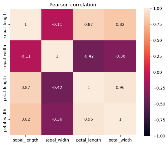
In the heatmap values above 0.59 can be considered as “solid” correlation. Petal length is strongly correlated with petal width along with sepal length, while sepal width is not strongly correlated with any other variable.
Scatterplots
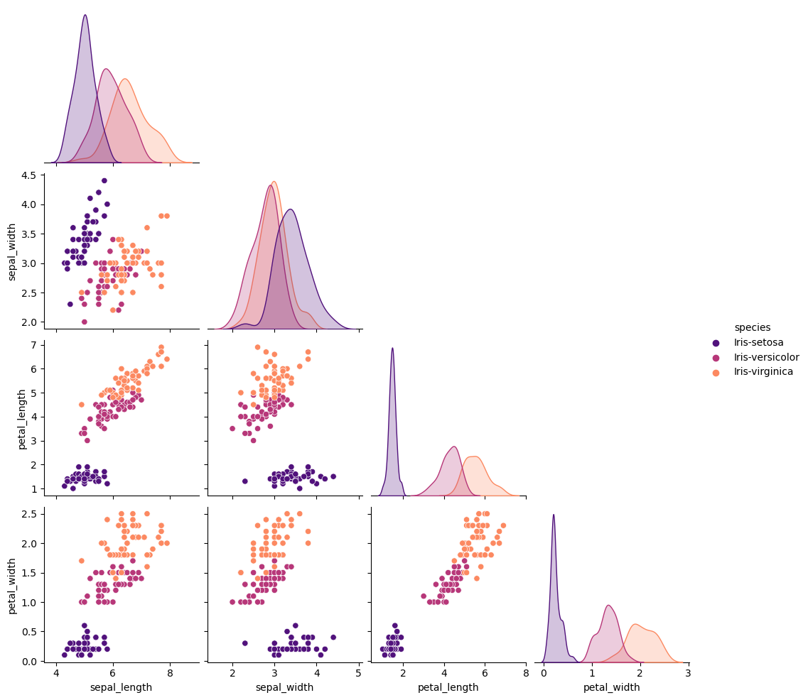
The pairplot shows the relationship between all pairs of features, with colors for each Iris species.
Petal length vs. petal width: the strong positive correlation seen in the correlation matrix (≈0.96) is clearly visible as an almost straight line of points.
Sepal length has moderate positive correlation with petal features, visible as slanted clouds.
Sepal width shows weaker or even negative correlations, confirmed by the scattered patterns.
Setosa is perfectly separated from the other species in petal features, while Versicolor and Virginica overlap.
This confirms the numerical correlation results and visually highlights which features best discriminate the species.
About scatterplots:
Classification
Normality test:
Feature: sepal_length
  Iris-setosa  | W=0.978, p=0.45950 | Normal ✅
  Iris-versicolor | W=0.978, p=0.46474 | Normal ✅
  Iris-virginica | W=0.971, p=0.25831 | Normal ✅

Feature: sepal_width
  Iris-setosa  | W=0.969, p=0.20465 | Normal ✅
  Iris-versicolor | W=0.974, p=0.33798 | Normal ✅
  Iris-virginica | W=0.967, p=0.18090 | Normal ✅

Feature: petal_length
  Iris-setosa  | W=0.955, p=0.05465 | Normal ✅
  Iris-versicolor | W=0.966, p=0.15848 | Normal ✅
  Iris-virginica | W=0.962, p=0.10978 | Normal ✅

Feature: petal_width
  Iris-setosa  | W=0.814, p=0.00000 | Not normal ❌
  Iris-versicolor | W=0.948, p=0.02728 | Not normal ❌
  Iris-virginica | W=0.960, p=0.08695 | Normal ✅
I tested normality of distribution of features within each species with Shapiro=Wilk test.
sepal_length: 0 outliers
sepal_width: 4 outliers
petal_length: 0 outliers
petal_width: 0 outliers
I found some outliers.
sepal_length: Levene stat=6.35, p=0.00226
sepal_width: Levene stat=0.65, p=0.52483
petal_length: Levene stat=19.72, p=0.00000
petal_width: Levene stat=19.41, p=0.00000
The Levene test tests the null hypothesis that all input samples are from populations with equal variances.Only sepal width is different than other features, when variances are compared.
sepal_length: ANOVA F=119.26, p=0.0000000000
sepal_width: ANOVA F=47.36, p=0.0000000000
petal_length: ANOVA F=1179.03, p=0.0000000000
petal_width: ANOVA F=959.32, p=0.0000000000
sepal_length: Kruskal H=96.94, p=0.0000000000
sepal_width: Kruskal H=62.49, p=0.0000000000
petal_length: Kruskal H=130.41, p=0.0000000000
petal_width: Kruskal H=131.09, p=0.0000000000
Before running ANOVA, I checked for outliers and normality. A few extreme values were found in sepal width, but they are consistent with real biological variation and not obvious data entry errors. Since ANOVA is sensitive to outliers and non-normal distribution of data, I also verified the results with the Kruskal–Wallis test, which is more robust to non-normality and extreme values. Both tests agreed, so I kept the outliers in the analysis. ANOVA and Kruskal–Wallis tests produced very small p-values (< 0.00001), indicating strong evidence against the null hypothesis of equal group means. This confirms that at least one species differs significantly from the others.
Tukey HSD results for sepal_length:

        Multiple Comparison of Means - Tukey HSD, FWER=0.05
===================================================================
     group1          group2     meandiff p-adj lower  upper  reject
-------------------------------------------------------------------
    Iris-setosa Iris-versicolor     0.93   0.0 0.6862 1.1738   True
    Iris-setosa  Iris-virginica    1.582   0.0 1.3382 1.8258   True
Iris-versicolor  Iris-virginica    0.652   0.0 0.4082 0.8958   True
-------------------------------------------------------------------

Tukey HSD results for sepal_width:

         Multiple Comparison of Means - Tukey HSD, FWER=0.05
=====================================================================
     group1          group2     meandiff p-adj  lower   upper  reject
---------------------------------------------------------------------
    Iris-setosa Iris-versicolor   -0.648   0.0 -0.8092 -0.4868   True
    Iris-setosa  Iris-virginica   -0.444   0.0 -0.6052 -0.2828   True
Iris-versicolor  Iris-virginica    0.204 0.009  0.0428  0.3652   True
---------------------------------------------------------------------

Tukey HSD results for petal_length:

        Multiple Comparison of Means - Tukey HSD, FWER=0.05
===================================================================
     group1          group2     meandiff p-adj lower  upper  reject
-------------------------------------------------------------------
    Iris-setosa Iris-versicolor    2.796   0.0 2.5922 2.9998   True
    Iris-setosa  Iris-virginica    4.088   0.0 3.8842 4.2918   True
Iris-versicolor  Iris-virginica    1.292   0.0 1.0882 1.4958   True
-------------------------------------------------------------------

Tukey HSD results for petal_width:

        Multiple Comparison of Means - Tukey HSD, FWER=0.05
===================================================================
     group1          group2     meandiff p-adj lower  upper  reject
-------------------------------------------------------------------
    Iris-setosa Iris-versicolor    1.082   0.0 0.9849 1.1791   True
    Iris-setosa  Iris-virginica    1.782   0.0 1.6849 1.8791   True
Iris-versicolor  Iris-virginica      0.7   0.0 0.6029 0.7971   True
-------------------------------------------------------------------
Post-hoc Tukey test confirmed that the species are different from each other in every feature.
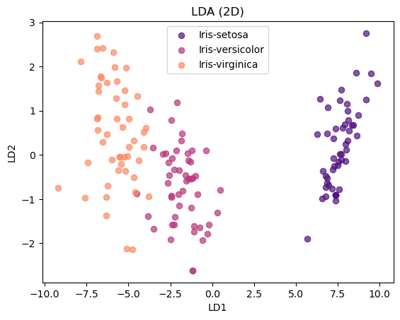
LDA reduces the 4D Iris dataset to 2D by finding axes that maximize species separation. The scatterplot of LD1 vs. LD2 shows that Setosa is perfectly separated, while Versicolor and Virginica overlap partially. This confirms that petal features dominate separation, and LDA effectively summarizes class structure.
Cross-validation:
Cross-validated accuracy:
LogisticRegression | CV Acc: 0.953 ± 0.045
             LDA | CV Acc: 0.973 ± 0.039
    DecisionTree | CV Acc: 0.953 ± 0.034

Held-out test performance:
LogisticRegression | Test Acc: 0.921
                 precision    recall  f1-score   support

    Iris-setosa      1.000     1.000     1.000        12
Iris-versicolor      0.857     0.923     0.889        13
 Iris-virginica      0.917     0.846     0.880        13

       accuracy                          0.921        38
      macro avg      0.925     0.923     0.923        38
   weighted avg      0.923     0.921     0.921        38

             LDA | Test Acc: 1.000
                 precision    recall  f1-score   support

    Iris-setosa      1.000     1.000     1.000        12
Iris-versicolor      1.000     1.000     1.000        13
 Iris-virginica      1.000     1.000     1.000        13

       accuracy                          1.000        38
      macro avg      1.000     1.000     1.000        38
   weighted avg      1.000     1.000     1.000        38

    DecisionTree | Test Acc: 0.895
                 precision    recall  f1-score   support

    Iris-setosa      1.000     1.000     1.000        12
Iris-versicolor      0.800     0.923     0.857        13
 Iris-virginica      0.909     0.769     0.833        13

       accuracy                          0.895        38
      macro avg      0.903     0.897     0.897        38
   weighted avg      0.900     0.895     0.894        38
I compared three classification models on the Iris dataset: Logistic Regression, Linear Discriminant Analysis (LDA), and a Decision Tree.
To estimate general performance, I used 5-fold stratified cross-validation. The mean and standard deviation of accuracy across folds show the stability of each model.
I trained each model on the training set (75% of data) and evaluated it on a held-out test set (25%).
For each model, I reported:
- Overall test accuracy. - A detailed classification report (precision, recall, F1-score). - A confusion matrix to visualize misclassifications.
The best accuracy was reached with LDA.